In part 16, we introduced RARS, the Robot Auto Racing Simulator. We talked about the clever and simple tyre-friction model in RARS and gave a terse presentation of its details in the big table in the article. Here, we'll explain in a little more detail why the model is cool.
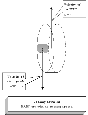
First, consider RARS' idea of a tyre when there is no steering applied. In the following diagram, we look down on a RARS tyre from above, using " X-Ray Vision" to see the contact patch:
There are only two interesting quantities at this point: the velocity of the car with respect to the ground, and the velocity of the contact patch with respect to the car. If there is no power, braking, or cornering applied, then these two vectors are equal and opposite in other words, the velocity of the contact patch with respect to the ground is zero. In general, if you have a velocity of some thing, any thing, with respect to the car and you have the velocity of the car with respect to the ground, all you have to do to get the velocity of the thing with respect to the ground is add the vectors, and we show how to add vectors immediately below. You eliminate the middleman - the car - by so doing. This is relativity, not the Einstein kind, but the Galileo kind-hence the title of this article. In the Einstein kind of relativity, you correct the vector sum with some quantities depending on the speed of light, a constant, and this is not relevant for auto racing because the speeds are so low compared to the speed of light, which is about 670 million miles per hour.
What happens when you apply a little steering input? Look at the next diagram.
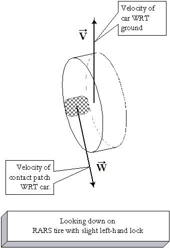
The velocity of the contact path with respect to the car,  ,
gets a little angle-the slip angle or the grip angle, as I called it in part 10
of the Physics of Racing.
still points directly back along the plane of the tyre, and the velocity of the
car with respect to the ground,
,
gets a little angle-the slip angle or the grip angle, as I called it in part 10
of the Physics of Racing.
still points directly back along the plane of the tyre, and the velocity of the
car with respect to the ground,  ,
still heads forward, that is, up on the page, at least for an instant. To
find out the velocity of the contact patch with respect to the ground,
,
still heads forward, that is, up on the page, at least for an instant. To
find out the velocity of the contact patch with respect to the ground,  , we add the vectors
and , just as before, but now there's an intervening angle. Here's
the procedure for adding the vectors: Transport one of them, without changing
its direction, so that its tail touches the head of the other one. It turns out
that not all kinds of vectors can be transported like this, but velocity in this
context is one of the kinds that we can freely transport. We'll transport
over to the head of ,
as in the following diagram:
, we add the vectors
and , just as before, but now there's an intervening angle. Here's
the procedure for adding the vectors: Transport one of them, without changing
its direction, so that its tail touches the head of the other one. It turns out
that not all kinds of vectors can be transported like this, but velocity in this
context is one of the kinds that we can freely transport. We'll transport
over to the head of ,
as in the following diagram:
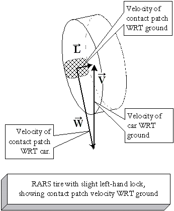
Draw a new vector from the tail of to
the head of in
its new location. This new, little vector is defined as the vector
sum, ,
drawn from the tail of one to the head of the other. Note it would have the same
direction and length if it were drawn from the tail of to
the head of .
Because of this fact, we can write the following equation:
= + = +
This procedure for adding vectors works even when the vectors are collinear, in which case the triangle is flat, the opposite corners coincide, and the vector sum is zero-the mathematically unique vector zero. It also turns out that this procedure has a very simple equivalent in algebraic form. To do computations, we need to represent vectors with numbers. To do so, we measure the length of the projection of the vector against the axes of a coordinate frame, as in the following diagram:
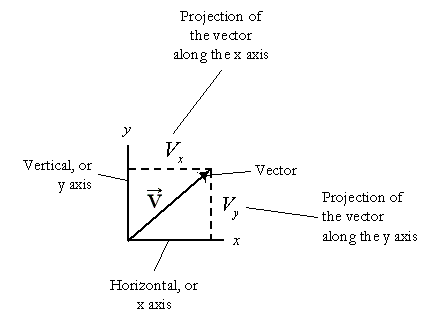
So, we get just what we need: numbers, also called components
because they are the component parts that make up the perpendicular, independent
projections of the vector. Numbers, in general, are also called scalars
since they can be used to scale vectors. In general, we'll get three numbers for
any vector in a 3D world, and two numbers in a 2D world. In either case, adding
vectors is trivial. If we write
= (Vx, Vy, Vz) and = (Wx, Wy, Wz), then
+
= (Vx + Wx + Vy + Wy + V z + Wz)
Just add them up componentwise. Couldn't be easier. I'll leave it to you to show that the head-to-tail method is equivalent to the numerical add-'em-up-componentwise method.
Let's go back to the tyres. Here's what makes RARS' model so clever: It's
undeniable that the contact patch moves with respect to the ground if we assume
that it continues to move in the circumferential direction with respect to the
wheel and the car. We can summarize all the complex motion of the contact patch
in a single velocity
and we can approximate our friction model so that it depends only on the
magnitude of .
This is a simpler model than the one presented in part 10, but also potentially
less accurate. Let's review that one briefly. Again, looking at the contact
patch from above, as if by X-Ray vision:
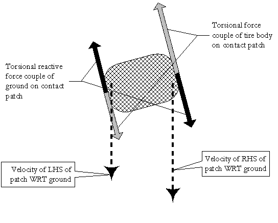
In the diagram above, we're looking at a wheel steered slightly to the left of the direction of travel. Assuming that there's a little acceleration in addition to the steering, both sides of the contact patch move backwards with respect to the ground. The left-hand side (LHS) of the patch moves a little more slowly than the right-hand side (RHS) because the RHS crabs around the corner. The wheel, through the carcass of the tyre, twists the patch to the left, generating a force couple illustrated by the grey arrows. The ground resists, through friction, producing the right-twisting, restoring, force couple in black. Since the patch continues to twist leftward with respect to an inertial reference frame in a steady-state turn, the grey couple must be a little larger than the black one.
This model is not by any means complete, and it's already MUCH more complex
than the RARS model, which does a decent job in practice. RARS computes just
one quantity, the vector ,
and accounts for all forces and torques on the tyre through that one variable.
The advantages of the approach, when it comes to computer simulation, are
The limitations, of course, are that RARS cannot account for detailed tyre physics and important effects like suspension geometry and dynamics, so the whole scheme trades off accuracy for simplicity. However, as a quick-and-dirty approximation, it's remarkably effective.